cs7641-PointCloudSegmentation.github.io
CS7641 Project Proposal
3D Data Clustering and Segmentation for Indoor Environment
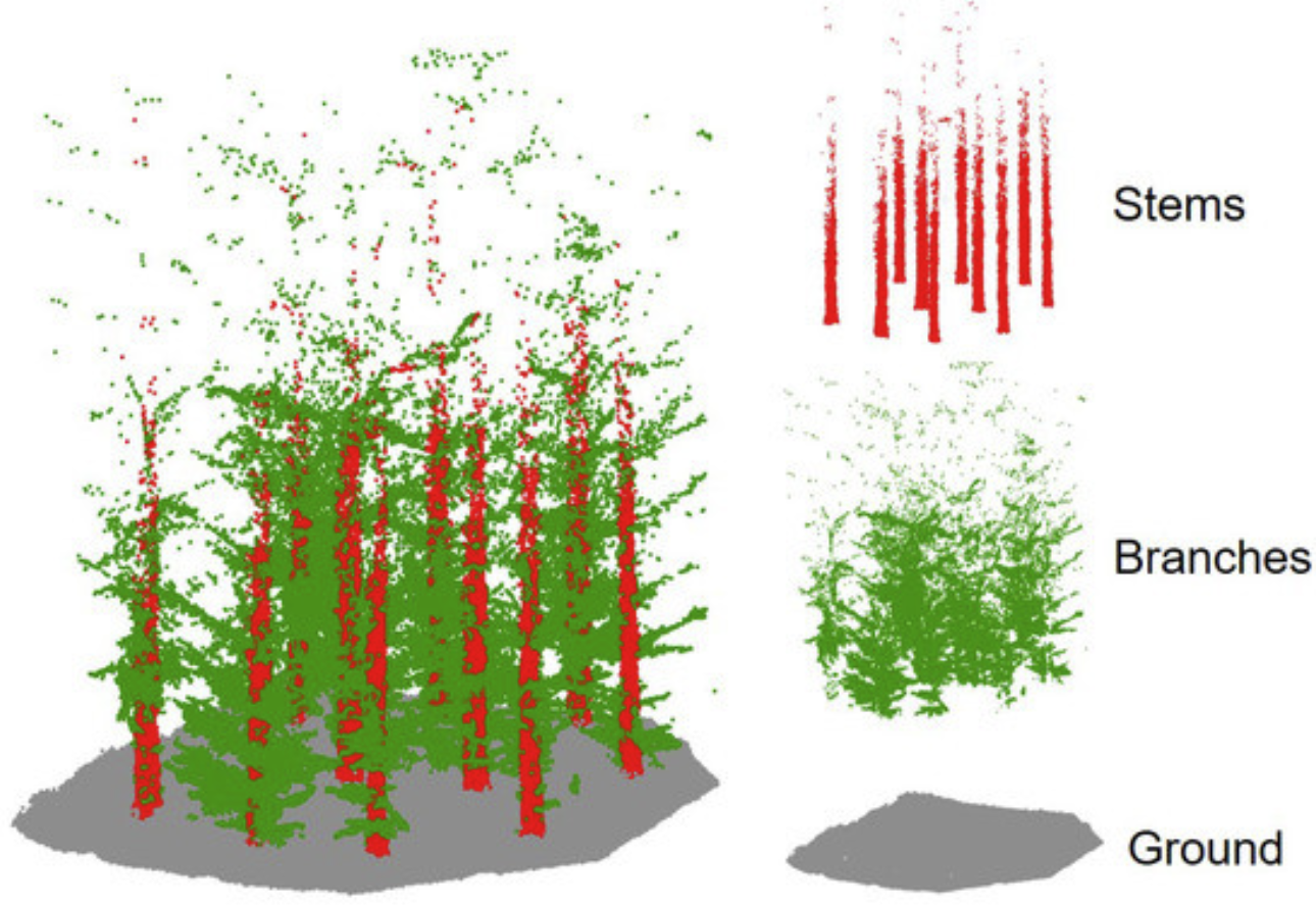
Figure 1. Example of point cloud processing result from [8]
Team members
Kaylah Facey, Madison Manley, Seongyong Kim, Yosuke Yajima
Introduction & Background
With the advancement of sensor technology, there is an explosion of 3D data, called point clouds, that is captured using 3D depth cameras and LiDAR sensors. Point clouds are useful in diverse applications including self-driving cars, surveys of infrastructure monitoring, and indoor mappings for buildings. Compared to research in 2D images, processing 3D data is a relatively new technology that uses machine learning to classify and detect objects. Using 3D data is advantageous as it is difficult, slow, and error prone to reconstruct 3D spaces using 2D images.
Problem Statement
In civil engineering, point clouds are being used to create indoor mapping building models, as this method is significantly faster and more accurate compared to creating models by hand. However, once a point cloud is collected using LiDAR or 3D depth cameras, it takes a considerable amount of time and labor intensive work to process the point clouds into a usable model. Automating point cloud processing and reducing the processing time is very critical for applications that require point clouds to be processed immediately. In this project, we want to demonstrate how machine learning can be used to automate and improve point-cloud processing time.
Methods
1. Dataset and Pre-processing
Stanford 3D Indoor Space Dataset
We use the S3DIS dataset which contains 3D room scenes for semantic segmentation[3]. It contains point clouds of 276 rooms in 6 buildings, where each point is labeled in one of the 13 categories (wall, chair, table etc.).

Figure 2. S3DIS dataset [3]
Pre-processing
To clean up this dataset, all points are rounded to first decimal place and downsampled to reduce the size of overall point cloud data. Additionally, all points are centered to align coordinates of point cloud objects. It’s a very large dataset, so for the scope of this project, we are focusing on the first 2 buildings. Based on the ground truth provided, we prepare labeled point clouds for both semantic and instance segmentation (figure 3).

Figure 3. A sample of (a) semantic label, (b) instance label. Note that the same objects like a wall and a chair in the semantic label is distinguished and separated in the instance label.
Feature Selections
A point cloud has both geometry features (xyz coordiantes) and color features (rgb values). To search the optimal feature spaces, we applied the combination of PCA and a normalization, then compared each performance of the model. Also, we added features reflecting geometry natures, such as surface normals and curvature.
For training our deep networks, which requires more cleanly refined data, we separated rooms and assinged a id, to seperately perform the centering of the xyz cooridante per each room.

Figure 4. Data label sample: class id and room id
2. Point Cloud Clustering via Unsupervised Learning
Clustering using Class Labels
We attempted K-Means and GMM clustering with our centered dataset preprocessed in several different ways: 1) the original data, 2) the normalized data, 3) the data with 3 PCA components, 4) the normalized data with 3 PCA components. We processed and clustered the data one room at a time to relate the points in each room to eachother and simplify the clustering task. For each room, we tried several different values of K and chose the one that resulted in the highest homogeneity with the ground-truth labels. The reason we clustered on homogeneity as opposed to Mutual Information or the Rand Index is because the points in the s3dis dataset are labeled by classes that can each correspond to multiple objects that would not necessarily be clustered together. For example, a chair on one end of a room would probably not be clustered with a chair on the other end, though they would both be labeled as a chair. Mutual Information and the Rand Index penalize clustering that divides classes, but we care more about how well clusters are divided into classes than about whether classes are divided into different clusters. We limited the number of clusters to between the number of ground-truth labels present in that room to double that number. We want to ensure that each label is theoretically represented at least once, and we limited the number to double the number of ground-truth labels to limit the time required to perform clustering and prevent super small, trivially homogenous clusters. For a single room, homogeneity scores can be visualized:
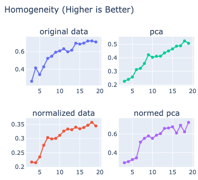
Figure 5. Homogeneity from 3 to 20 clusters for Area 1 Conference Room 1
Then we calculated the average homogeneity and found that for both K-Means and GMM, the most homogenous (43% for K-Means and 65% for GMM) clusters resulted from using the normalized data. To further analyze the normalized data clustering, we found the proportions of all ground-truth labels in each cluster in the dataset and graphed those percentages to show how strongly the ground-truth labels were clustered:

Figure 6. K-Means Homogeneity Analysis

Figure 7. GMM Homogeneity Analysis
The most representative ground-truth label for each cluster forms roughly 40-100% of that cluster, with many forming over 80% of their cluster. Ground-truth labels are significantly correlated with clusters, supporting our 65% average homogeneity score. We also did a visual comparison of ground-truth labels to cluster labels for 3 rooms:
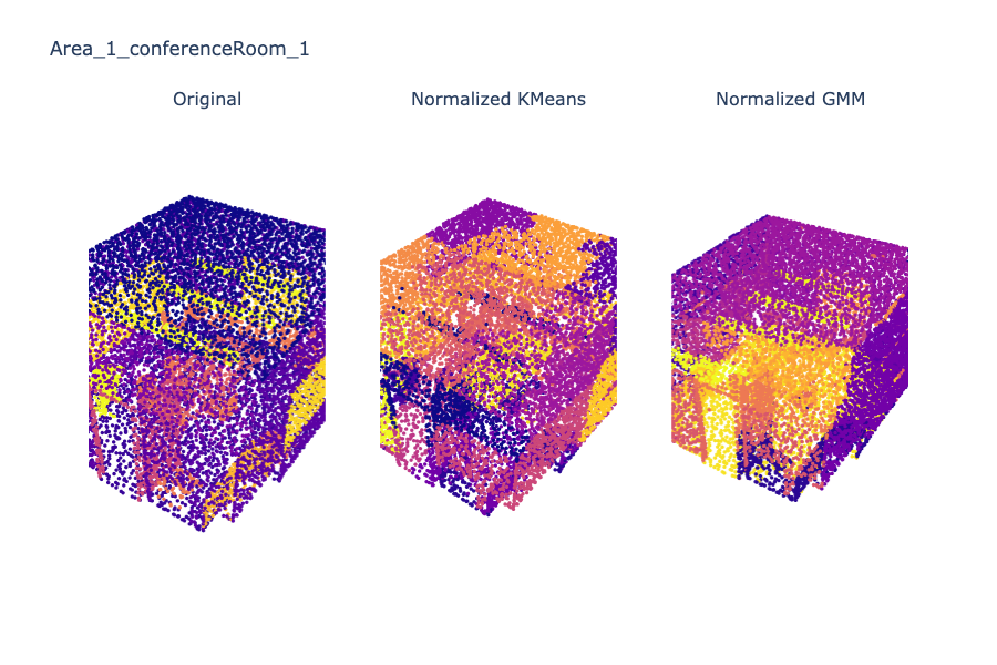
Figure 8. Area 1 Conference Room 1
The main features of the room are visible in all three images, showing the correlation between the clustering and the ground-truth labels. We can see that the KMeans clusters are more patchy; the GMM clusters more closely approximate the ground-truth labeling. In particular, the roof, yellow bars, orange table and chairs, and most of the doorframe are delineated by GMM where in K-Means they are broken up by many different clusters.
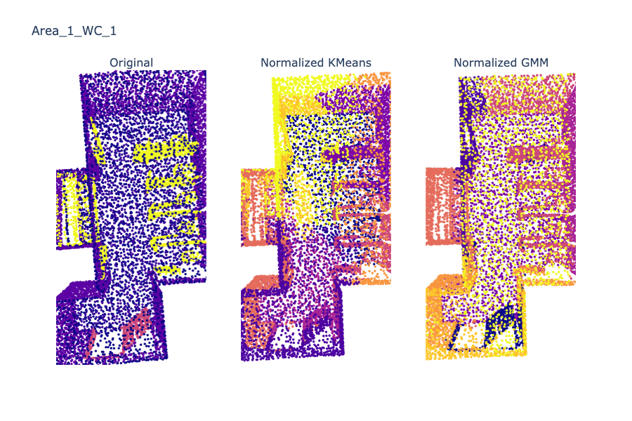
Figure 9. Area 1 WC 1
Again, note that both K-Means and GMM have clearly delineated stall lines, though again, GMM’s lines are cleaner.
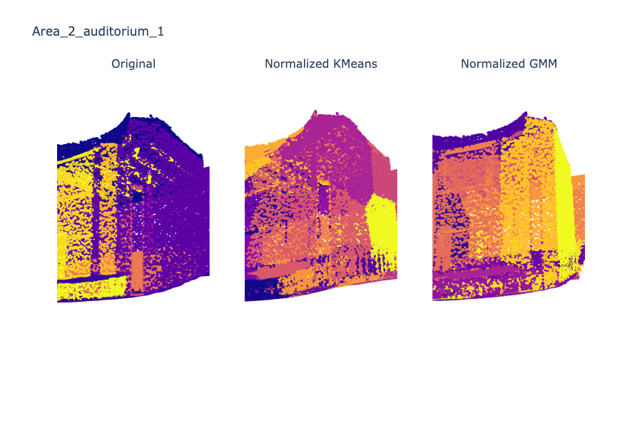
Figure 10. Area 2 Auditorium 1
Again, the lines under the ceiling are visible in all three renderings, and GMM provides better definition to the walls than K-Means.
Clustering Using Instance Labels
The S3dis dataset is labeled in terms of classes, such that multiple objects may exist for one class (e.g, a conference may have multiple objects all of whose point labels would be ‘chair’). After processing the dataset to find the instance labels, we decided to analyze clustering performance using the instance labels rather than the class labels. Using instance labels allows us to analyze our data with more sophisticated metrics than Homogeneity, such as the Adjusted Rand Index and the Fowlkes-Mallows Index. This is because the multiple objects in a class may not be close together and could be placed in different clusters for that reason. The points in a single instance of a class, however, should generally be clustered together as they are expected to be close together by virtue of belonging to the same object.
As with clustering using class labels, we first preprocessed the data in several ways to get a better idea of what the best preprocessing to use in clustering is. We used the Original Data, Normalized Data, the data as PCA Components, and the data as Normalized PCA Components. We clustered a subset of the data for each preprocessing method and compared the results to determine which methods to use to cluster the rest of the data.
For the subset of data, each room was clustered using multiple values of k to help determine the best value of k. We found the number of instance labels present in each room and tried k values between half that number and 1.5 times that number, incrementing in step sizes of 1/10th the range between the min and max values.
We first found correlations between unsupervised metrics and supervised metrics for all preprocessing methods and found that for all methods, the supervised Adjusted Rand Index and Fowlkes-Mallows Index were more highly correlated with the unsupervised Silhouette Score and Davies-Bouldin Index than the supervised Homogeneity Score and the Adjusted Mutual Index, e.g:
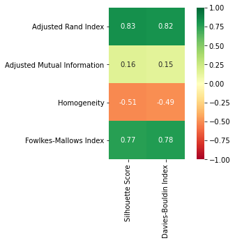
Figure 11. K-Means Original Data Supervised-Unsupervised Correlation
We also found that the Silhouette Score was generally a better predictor of the supervised scores than the Davies-Bouldin Index, and where the DBI had a higher correlation with unsupervised scores, the difference was very small. We therefore decided to use the Silhouette Score as our unsupervised metric of choice to compare k values.
Again on the small subset of training data, for each room we found the best silhouette score and plotted the Adjusted Rand Index at that k:
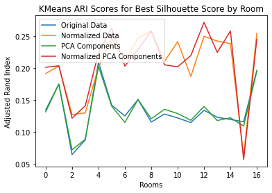
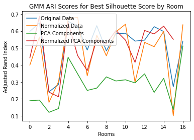
Figure 12. Compare Preprocessing Methods using ARI Scores
Examining those results, we saw no advantage to using PCA Components and decided to cluster the rest of our Area 1 data using only the Original Data and Normalized Data.
In addition to the k-selection we used for the small subset of data, for clustering on all of Area 1 we fine-tuned our k value by finding the k with the highest silhouette score and re-clustering the dataset with k values between the next lowest k and the next highest k we had already tried, with a step size of 1/10th the previous step-size. For example, if we had clustered in increments of 100 from 100 to 900 and the best silhouette score was found at the 600 value, we would cluster for k values 500 to 700 in increments of 10. We selected k using the silhouette score rather than a supervised metric because we wanted to preserve the unsupervised nature of clustering and use supervised scores only for analysis and validation.
Analyzing the clustering of Area 1, we found that K-Means produced better results with Normalized Data. GMM’s scores were comparable between Normalized and Original Data, but the Original Data scores were more stable:
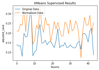
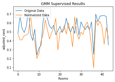
Figure 13. Compare Preprocessing Methods using ARI Scores
We also compared all supervised metrics for GMM (Original Data) and K-Means (Normalized Data) and saw that GMM outperformed K-Means in every respect except for Homogeneity:
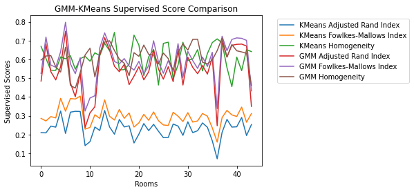
Figure 14. Compare Area 1 Supervised Metrics for KMeans and GMM
With that information, we then clustered the Area 2 data using only the Original Data for GMM and only the Normalized Data for K-Means and analyzed the results. Again, GMM mostly outperformed K-Means, though GMM results had much more variation than K-Means, and K-Means homogeneity was the best-performing metric overall:
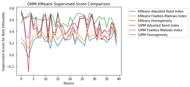
Figure 15. Compare Area 2 Supervised Metrics for KMeans and GMM
Finally, we analyzed the results for Area 1 and Area 2 together. The combined supervised scores graph shows clearly that while K-Means scores show roughly the same amount of variance in Area 1 and Area 2, GMM scores are much more varied for Area 2:
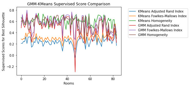
Figure 16. Compare Area 1 and 2 Supervised Metrics for K-Means and GMM
We also analyzed the cluster purity and label purity of the combined data. Cluster purity was measured as follows: we divided each cluster into the instance labels of its points and found the instance label with the most points. We then took its percentage of the cluster as the cluster purity. Label purity was measured similarly: we divided the points of each instance label into all the clusters they belonged to and took the percentage of the cluster that held the most points of that instance label. To chart the scores for each room, we divided the purity scores into 10 buckets from [0%, 10%) to [90%, 100%) and an 11th bucket for 100%. We sized each point on the graph by the number of clusters in each bucket, and the center of the points is the average cluster purity for that bucket:
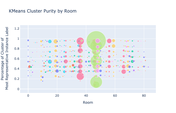

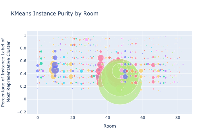
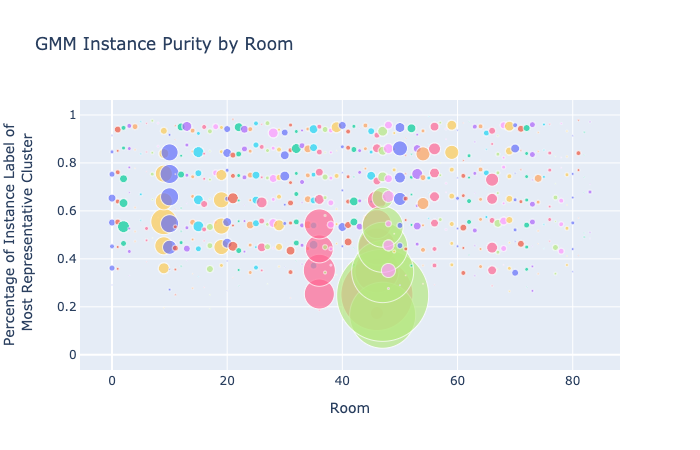
Figure 17. Compare Cluster and Instance Purity for KMeans and GMM
For cluster purity, both GMM and K-Means show more clusters at the top and bottom of the graph than in the buckets in between, suggesting that clusters are either very strongly or very weakly correlated with instance labels. It’s possible that when instance labels aren’t clustered into a very representative cluster, they are more or less randomly assigned.
For instance purity, GMM scores are clustered somewhat higher in the graph than for K-Means, though both methods have a lot of variation in scores. One of the rooms (light green) has a lot of instance labels that aren’t strongly represented by a cluster in either method.
Finally, we compared k values for GMM and K-Means (again, the chosen k value for each room is the k yielding the highest silhouette score):
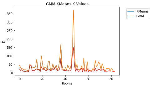
Figure 18. Compare K-Means and GMM K Values
Most rooms had K values under 100 for both KMeans and GMM. GMM scores vary wildly between roughly the same value as KMeans to several times higher; nowhere is that more obvious than at the spike in the middle of the graph, where the KMeans k is around 150 and GMM sets k to over 350. GMM, then, was able to improve silhouette scores (and supervised scores, correspondingly) by increasing k. This suggests that GMM was better able to distinguish between instances than K-Means.
To better compare GMM and K-Means, we visualized the clustering results:
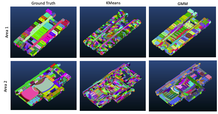
Figure 19. Intance segmentation results
Above figure shows our results of the instance clustering. In aspect of distinguishing each building element, GMM outperforms Kmeans; GMM is more likely to segments each instance preserving a planarly shape, whereas those of Kmeans are over-divided even with the objects on the same plane.
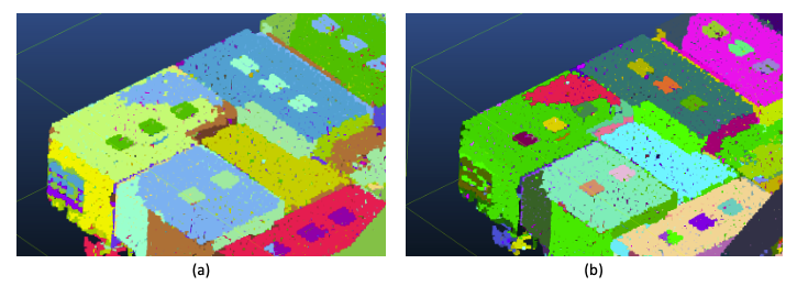
Figure 20. (a) GMM, and (b) GMM with DBSCAN. Note that each hole in the ceiling change to different colors, indicating that they are distinguished as the different intance label.
We found that DBSCAN with appropirate parameters could be a good solution for further distinguishing each instance that has been already segmented. For a point cloud, DBSCAN in nature is not a proper algorithms for the instance clustering as its criteria of the data density seems to be all similar on building elements. However, by setting the point distance parameter close to the point cloud resolution and the minimum point number parameter to 1, it works as to find a connected component in the 3D space. With an advantage of this properties, we additionally sub-divided our clustering reults and compare the clustering performance.
3. Point Cloud Semantic Segmentation via Supervised Learning
Supervised learning will be used to classify different types of objects. We developed a model named, Dynamic Graph PointNet (DGCNN), that combined the graph based deep learning method Dynamic Graph CNN (DGCNN) and PointNet to classify objects in a building dataset. In this neural network, multi-layer perceptron of PointNet and DGCNN are concatenated into one multi-layer perceptron. This combination aims to combine learned featured from PointNet and DGCNN to predict object semantic labels such as floors, ceilings, and walls from the building dataset.
As deep learning for 3D point cloud classification is an active research area, we want to compare DGCNN with conventional methods [8]. Therefore, as a point of comparison, we also plan to evaluate models using Random Forest.
Results for DGPointNet
The PointNet, DGCNN, and DGPointNet model are trained and tested with all data (Area1 to Area 6) in S3DIS dataset. Each test set and training set contains different rooms, and all data is labeled (default semantic segmentation labels). In this experiment, Area 5 is used to test our models and all other areas are used to train our models. The following plots show our training and validation results.
By comparing the training and validation, training loss is converged to minimum point and the validation loss shows fluctuating results after the loss is converged to minimum point. Training and validation accuracy both improved as the number of training and validation epochs increased. Intersection of Union (IoU) is used to evaluate performance of the deep learning models.
All models used in the following diagram has a same training parameters as shown below.
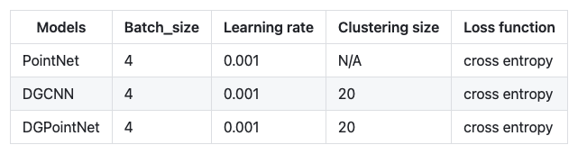
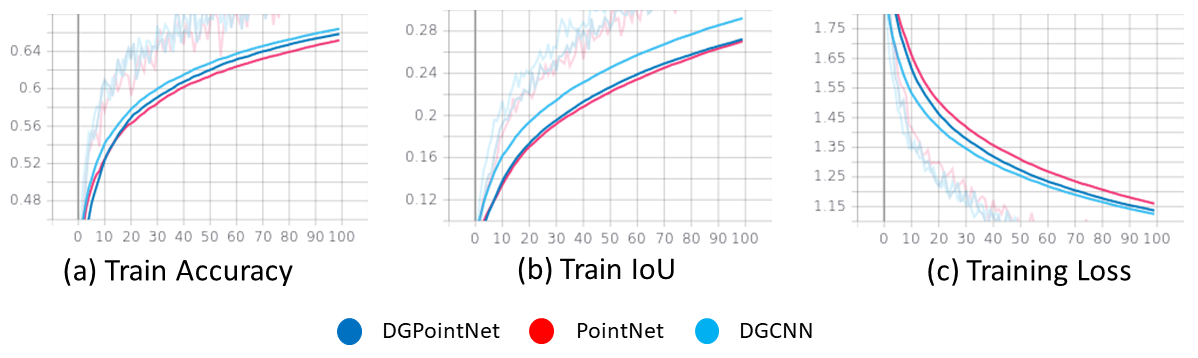
Figure 21. Training Logs (accuracy, loss, and IoU)
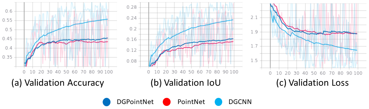
Figure 22. Validation Logs (accuracy, loss, and IoU)
Visual representations in point cloud data format are presented as follows. The left images are all ground truth labels and the right images are all predictions by our deep learning models.

Figure 23. Comparison between PointNet, DGCNN, and proposed models (DGPointNet) using example pointcloud data
Next, hyperparameter tuning was performed to improve our proposed method. Two regularization methods were used in this experiment, weight decay (l2 regularization) and adding a regularization developed by PointNet. The result shows that the proposed model is able to improve its validation accuracy and IoU metrics as described in the following diagram.
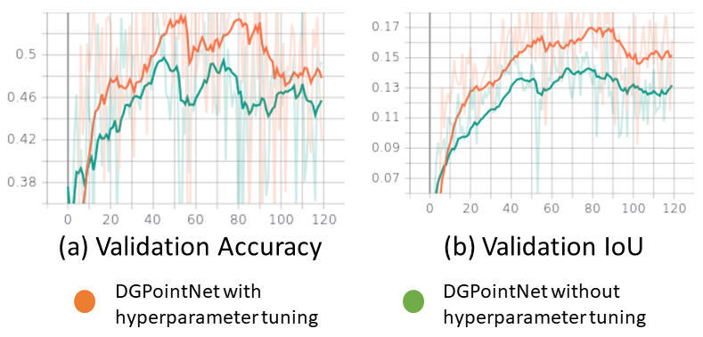
Figure 24. Hyperparameter Tuning with additional regularization terms.
Results for Random Forest
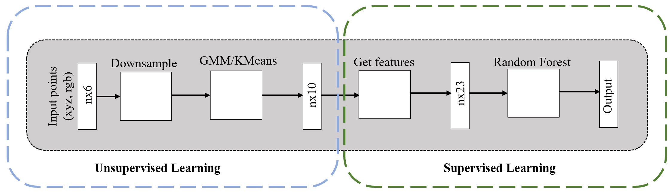
Figure 25. Block Diagram of Random Forest Model
As a point of comparison to DGCNN, we have used random forest for 3D point cloud classification. Area 1 was used to train the random forest model and Area 2 was used to test the model. To do this, features were extracted from the point cloud xyz coordinates and RGB values to train the random forest model. Below are the following features that were extracted and used:
- eigenvalues
- surface normals
- curvature
- anisotropy
- eigensum
- linearity
- omnivariance
- planarity
- sphericity
- RGB intensity
A parameter study was first done on the number of k-nearest neighbors used to calculate the features and the number of trees used in the forest to find the best configuation of each random forest model. The feature importance was also found using mean decrease in impurity (MDI).
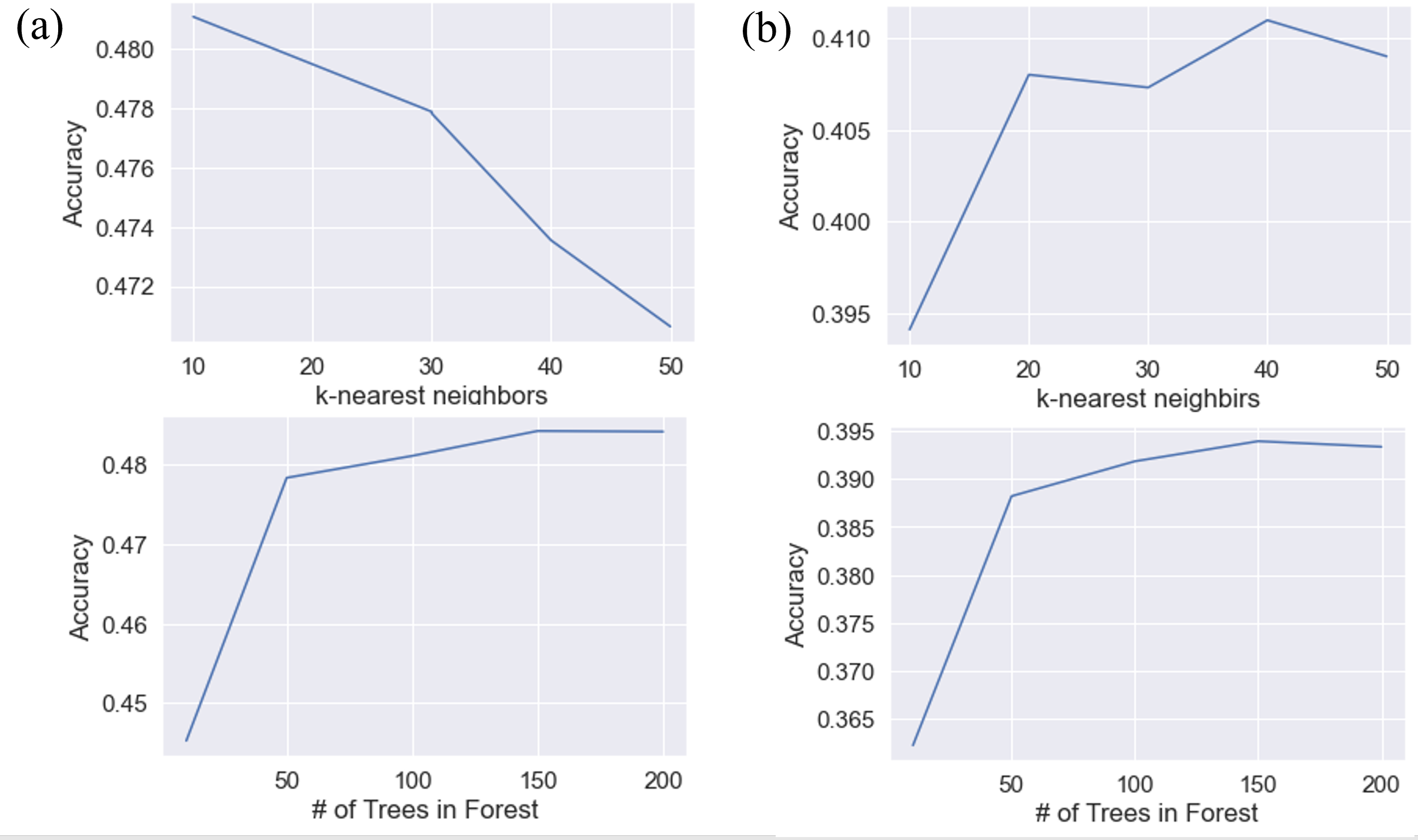
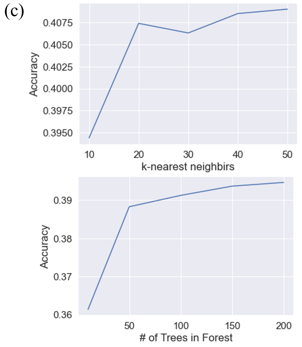
Figure 26. (a) Ground truth classification (b) Classification with Cluster Label (KMeans) (c) Classification with Cluster Label (GMM)

Figure 27. Feature Importance using MDI
Once the best configuration was found for each model, each model was tested using the Area 2 dataset. A confusion matrix and classification report was found for the 3 models to give us more information into what objects the models had trouble in classifying. We can see that the models had most trouble in classifying objects such as walls, floors, and tables and could more easily classify objects such as clutter, boards, and sofas. It is interesting to note that even though the overall accuracy of the model decreased when using the cluster labels from our unsupervised models, it slightly improved the classifcation of walls and floors. Our model DGPointnet is designed to to predict object semantic labels such as floors, ceilings, and walls from the building dataset which could be a potential reason why the accuracy is higher compared to random forest. The table below compares the highest accuracy each model achieved:
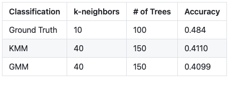
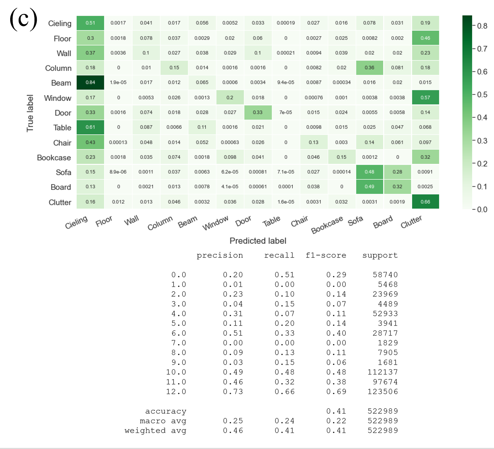
Figure 28. (a) Ground Truth classification (b) Classification with Cluster Label (KMeans) (c) Classification with Cluster Label (GMM)
Conclusion
Our project proposed unsupervised and supervised methods that group a point cloud into several clusters and predict semantic object labels.
In the unsupervised learning methods, we compared the performance of K-Means and GMM on clustering point cloud data and found that GMM outperforms K-Means in almost every way for both class-based clustering and instance-based clustering. After performing instance-based clustering, we further clustered the data using DBSCAN and found that we were able to more accurately predict instance labels that way.
In the supervised learning method, a deep learning model named DGPointnet is compared with other deep learning models such as PointNet and DGCNN. The results show that the proposed method performs better than PointNet architecture, while the DGCNN models perform a better result compared to our proposed method in terms of validation accurcy and IoU metrics. In terms of hyperparameter tuning, the weight decay and regularization techniques developed by PointNet prevent an overfitting issues by improving the validation result. We found that DGPointnet has a higher accuracy compared to random forest, which has the most trouble in classifying floors, ceilings, and walls.
Overall this project provided us an insight into machine learning and deep learning research related to 3D computer vision and point cloud processing.
References
[1] D. Maturana and S. Scherer, “Voxnet: A 3d convolutional neural network for real-timeobject recognition,” in2015 IEEE/RSJ International Conference on Intelligent Robotsand Systems (IROS), pp. 922–928, IEEE, 2015.
[2] C. R. Qi, H. Su, K. Mo, and L. J. Guibas, “Pointnet: Deep learning on point sets for 3dclassification and segmentation,” inProceedings of the IEEE conference on computervision and pattern recognition, pp. 652–660, 2017.
[3] I. Armeni, O. Sener, A. R. Zamir, H. Jiang, I. Brilakis, M. Fischer, and S. Savarese, “3dsemantic parsing of large-scale indoor spaces,” inProceedings of the IEEE Conferenceon Computer Vision and Pattern Recognition, pp. 1534–1543, 2016.
[4] S. Chen, C. Duan, Y. Yang, D. Li, C. Feng, and D. Tian, “Deep unsupervised learning of3d point clouds via graph topology inference and filtering,”IEEE Transactions on ImageProcessing, vol. 29, pp. 3183–3198, 2019.
[5] Y. Yang, C. Feng, Y. Shen, and D. Tian, “Foldingnet: Interpretable unsupervised learningon 3d point clouds,”arXiv preprint arXiv:1712.07262, vol. 2, no. 3, p. 5, 2017.
[6] J. M. Biosca and J. L. Lerma, “Unsupervised robust planar segmentation of terrestri-al laser scanner point clouds based on fuzzy clustering methods,”ISPRS Journal ofPhotogrammetry and Remote Sensing, vol. 63, no. 1, pp. 84–98, 2008.
[7] L. Zhang and Z. Zhu, “Unsupervised feature learning for point cloud understandingby contrasting and clustering using graph convolutional neural networks,” in2019International Conference on 3D Vision (3DV), pp. 395–404, IEEE, 2019.
[8] S.-L. F. R.-P. J. Cabo C, Ordóñez C and C.-J. AJ, “Multiscale supervised classificationof point clouds with urban and forest applications,”Sensors(Basel), vol. 19, 2019.3.
[9] Chen, Jingdao, Zsolt Kira, and Yong K. Cho. “LRGNet: Learnable Region Growing for Class-Agnostic Point Cloud Segmentation.” IEEE Robotics and Automation Letters 6.2 (2021): 2799-2806.
[10] Chen, J., Kira, Z., & Cho, Y. K. (2021). LRGNet: Learnable Region Growing for Class-Agnostic Point Cloud Segmentation. IEEE Robotics and Automation Letters, 6(2), 2799-2806.
***
Timeline
June 14
- project proposal due date.
June 18
- prepare, clean up, and preprocess the s3dis dataset.
- work on implementing unsuperviesed learning and supervised learning algorithm.
June 25
- Complete implementing algorithm and validate results using small dataset. s
- start implementing evaluation metrics and visualization code.
July 7 - Project midpoint report
- validate model using a large dataset and optimize the algorithm.
- start preparing base line models to compare the result against our proposed method.
- start writing a final report and prepare final presentation.
- complete implementing evaluation metrics.
August2 - Final prohect due date
- record final presentation video.
- complete final report.
- clean up and organize github repository.
Team Members’ Responsibility
Kaylah Facey
- GMM and K-Means clustering (class and instance labels) and analysis
- helper function to visualize point cloud results
Madison Manley
- point cloud classification algorithm using Random Forest method
- evaluation metrics and optimizing model
Seongyong Kim
- raw data processing
- DBSCAN and analysis
- Instance segmentation visualization
Yosuke Yajima
- raw data processing
- DGPointNet and evaluation metrics